The mathematical model

instead of a lead

The calculation of infection spreads is typically done using so-called SIR models and their extensions. The models are coupled systems of ordinary differential equations. By choosing different parameters, one determines the type of infectious disease under consideration. These are values such as probability of infection, duration of infection and size of the population. Spatial conditions and the actual movement of people do not enter into the calculations of SIR models. We calculate the spread of infection based on the movement of a crowd, which depends for its part on the geometry of the room.

We consider a crowd as a continuum, i.e. we make the (false) assumption that a crowd consists of infinitely many infinitesimally small particles. We demand mass conservation and we look for the fastest way out. These wishes are formulated in the form of partial differential equations, which are calculated approximately using finite element methods. As a result, we get a kind of probability distribution that indicates when and where how many people are and in which direction and how fast they are walking. Based on these results, agents are calculated that have properties such as infectious, infected, infectable or recovered.

In the future, the SIR model will also be calculated continuum-based. The main reason is that the calculation of the agents is very time-consuming and thus the simulation is no longer practical. Furthermore, we want to investigate the influence of ventilation in the room on the infection process, or make it investigable with the software.

1. Crowd dynamics

The model for the pedestrian motion in evacuation scenarios — called pFlow — has been developed in a series of projects that were launched 2012 by R. Axthelm (2016) and the industrial partner ASE AG. It is deduced from the pedestrian flow model by R. Hughes (2002) and relies on the following assumptions:

hypotheses

[H1] Persons want to reach the nearest exit.
[H2] Persons want to minimize their travel time.
[H3] The speed only depends on the density of the surrounding pedestrians.

The model describes the crowd as a continuum. The movement of the crowd follows physical laws as we would expect in a crowd. It is assumed that the crowd of pedestrians behaves rationally and follows the above hypotheses. The dynamics of the crowd is described by its density $\varrho$ and its velocity $u=(u_1,u_2)$ at a given time $t$ and location $(x,y)$ .

The governing equations are the continuity equation which states that the flow of pedestrians into a small region equals the accumulation or loss of the pedestrians in this region and the eikonal equation which computes the minimal amount of time required to travel to the exit where the speed $f=f(\varrho)$ only depends on the local densitiy of the crowd

eikonal-equation decision of walk direction

\begin{equation*}\large -|\nabla \Phi| = \frac{1}{f(\varrho)} \end{equation*}

velocity-field speed and walking direction of the crowd

\begin{equation*} u=−f(\varrho)\frac{\nabla \Phi}{|\nabla\Phi|} \end{equation*}

continuity-equation preservation of human mass

\begin{equation*}\large \varrho_t+\nabla\cdot(\varrho,u)=0 \end{equation*}

$f(\varrho)$ is a given function which relates density to speed. It is called fundamental diagram. There exist a lot of different propositions in the literature how it looks like, none of them is fully accepted, but some of them verify important scenarios. Figure 1 shows an example of a fundamental diagram (blue) that is given by

\begin{equation*} f(\varrho)=1-e^{-\gamma,\left(\frac{1}{\varrho}-1\right)},~\gamma=0.3 \end{equation*}

and the corresponding specific power $f(\varrho),\varrho$ (red). The specific power describes the flow rate given by the number of persons (mass) per time- and length-unit.

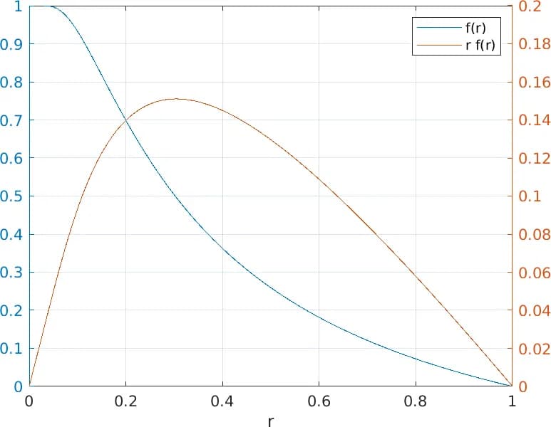Figure 1: fundamental diagram (blue) and specific power (red)

The scalar field $\Phi$ (Figure 2, left), also called cost-function, can be interpreted as a potential which describes the time it takes to reach the exit of the domain from a given location $(x,y)$. The preferred direction (Figure 2, right) then results from the direction of the respective negative gradient.

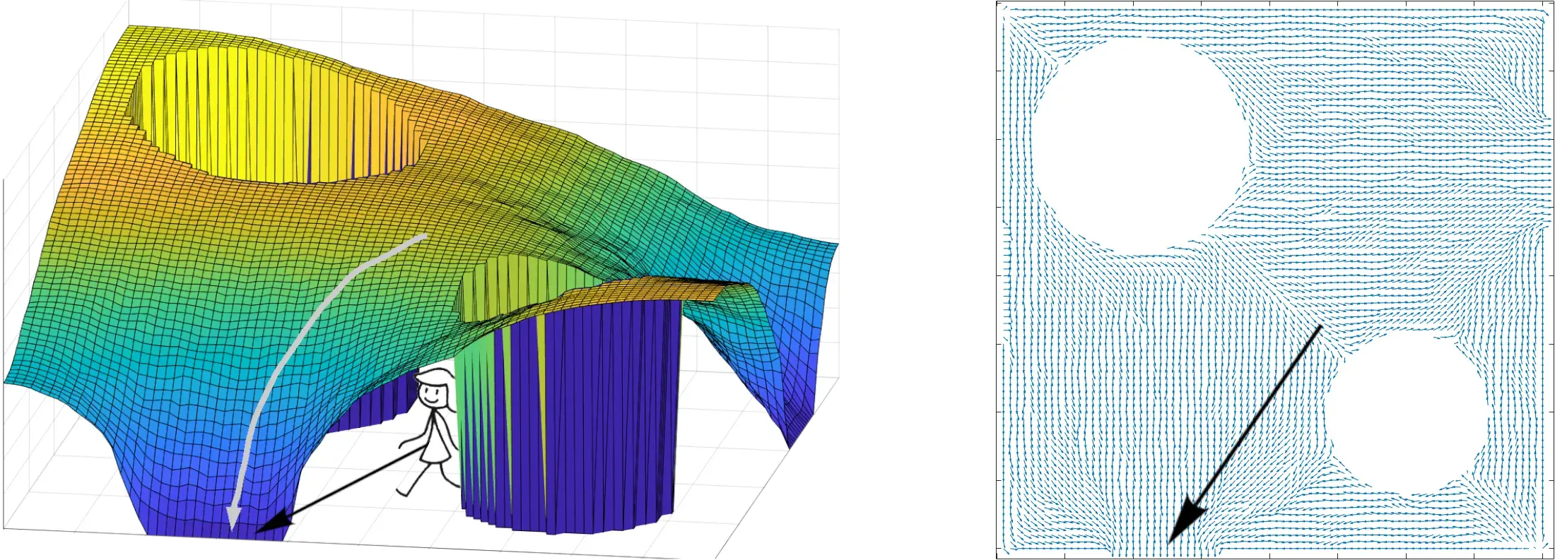Figure 2: Potential $\Phi$ (left) and resulting velocity field $u$ (right)

The examples in Figure 2 assume an empty room. High densities of people would dent the potential in the corresponding places.

2. Spread of infectious disease

The classical model to describe the spread of an infectious disease is a compartmental model called SEIR model. It was originally developed by W. Kermack and A. McKendrick (1927) as SIR-model. The population is divided into four compartments, the susceptible $S$, the exposed $E$, the infectious $I$ and the recovered $R$, and differential equations govern the flow of people from one compartment to the other: Let $S(t)$ be the individuals not yet infected, but susceptible to the disease, $E(t)$ the individuals exposed to the disease but not yet infectious, $I(t)$ the infected and infectous individuals and $R(t)$ the recovered (or died) individuals at time $t$. One usually assumes that the number of individuals is constant, that is

$$N=S(t)+E(t)+I(t)+R(t).$$

It is further assumed that each infectious individual has the same number of contacts per unit time, e.g. each infectious person meets 10 persons per hour. Not all of them are susceptible, but only $S(t)/N$ percent, e.g. 80%. Then each infectious person meets (at average) $10 \cdot 80% = 8$ susceptible persons. Not each contact leads to an infection, but only fractional part, e.g. only $15%$ of contacts leads to an infection, so in our example we get that each infectious person infects $15% \cdot 10 \cdot 80% = 1.2$ persons. One denotes the product of the probability of infection per contact and the contact rate (number of contact persons per unit time) with $\beta$ (e.g. here $15%\cdot 10=0.15$), and under these assumptions one obtains that the number of susceptible diminishes in each unit time by $−\beta S(t)/N(t)\cdot I(t)$:

$$S(t+1)−S(t)=−\beta\frac{S(t)}{N}I(t)$$

In the same way the other three differential equations are derived where $1/a$ is the average latency period (that is the time period between being exposed and being infectious), $\gamma$ is the average recovery rate (or $1/\gamma$ the mean infective period). We assume that the population in the considered time span is constant so that no new, susceptible individuals enter the system:

SEIR-Modell

$$\begin{aligned} E′(t)&=\beta\frac{S(t)}{N}I(t)−aE(t) \\ \\ I′(t)&=aE(t)−{\gamma}I(t) \\ \\ R′(t)&={\gamma}I(t). \end{aligned}$$

We see that the population flows from susceptible with rate $beta$, $S(t)/N$ to exposed, from exposed with rate a to infectious and from infectious with rate $\gamma$ to recovered. The basic reproduction number would be computed as $R_0=\beta/\gamma$ as fraction from exposition and recovery rate

The system has only one equilibrium state (if there are no new individuals entering the system) that no one is infected, that is $S+R=N$,$E=I=0$.

The classical SEIR model supposes that the contact rate is constant for each infected persons and that the four groups are everywhere homogeneously mixed such that the probability to meet a susceptible person is everywhere for everyone the same. The movements of people do not count. Therefore, the model does not allow to simulate local infections but only the global number of infections of the whole population. As we are interested in the interplay of pedestrian motion and spread of infections we develop a localised version of the SEIR model where for example infectious persons can locally accumulate and the time span that a susceptible persons spends close to an infected person counts.

Literature

Axthelm, R. (2016) Finite Element Simulation of a Macroscopic Model for Pedestrian Flow. In Knoop V., & Daamen W. (eds) Traffic and Granular Flow ‘15. Springer. Cham. https://doi.org/10.1007/978-3-319-33482-0_30

Hughes, R. (2002) A continuum theory for the flow of pedestrians. Transp. Res. Part B: Methodol. 36(6), 507–535 https://linkinghub.elsevier.com/retrieve/pii/S0191261501000157

Kermack, W. O., & McKendrick, A. G. (1927) A contribution to the mathematical theory of epidemics. Royal Sociaty 115, 772. https://doi.org/10.1098/rspa.1927.0118